One of the most important uses of textures is to vary material parameters across a surface. Previously, the finest granularity that we could get for material parameters is per-vertex values. Textures allow us to get a granularity down to the texel. While we could target the most common material parameter controlled by textures (aka: the diffuse color), we will instead look at something less common. We will vary the specular shininess factor.
To achieve this variation of specular shininess, we must first find a way to associate points on our triangles with texels on a texture. This association is called texture mapping, since it maps between points on a triangle and locations on the texture. This is achieved by using texture coordinates that correspond with positions on the surface.
Note
Some people refer to textures themselves as “texture maps.” This is sadly widespread terminology, but is incorrect. This text will not refer to them as such, and you are strongly advised not to do the same.
In the last example, the texture coordinate was a value computed based on lighting parameters. The texture coordinate for accessing our shininess texture will instead come from interpolated per-vertex parameters. Hence the prior discussion of the specifics of interpolation.
For simple cases, we could generate the texture coordinate from vertex positions. And in some later tutorials, we will. In the vast majority of cases however, texture coordinates for texture mapping will be part of the per-vertex attribute data.
Since the texture map's coordinates come from per-vertex attributes, this will affect our mesh topography. It adds yet another channel with its own topology, which must be massaged into the overall topology of the mesh.
To see texture mapping in action, load up the Material Texture tutorial. This tutorial uses the same scene as before, but the infinity symbol can use a texture to define the specular shininess of the object.

The Spacebar switches between one of three rendering modes: fixed shininess with a Gaussian lookup-table, a texture-based shininess with a Gaussian lookup-table, and a texture-based shininess with a shader-computed Gaussian term. The Y key switches between the infinity symbol and a flat plane; this helps make it more obvious what the shininess looks like. The 9 key switches to a material with a dark diffuse color and bright specular color; this makes the effects of the shininess texture more noticeable. Press the 8 key to return to the gold material.
The 1 through 4 keys still switch to different resolutions of Gaussian textures. Speaking of which, that works rather differently now.
Previously, we assumed that the specular shininess was a fixed value for the entire surface. Now that our shininess values can come from a texture, this is not the case. With the fixed shininess, we had a function that took one parameter: the dot-product of the half-angle vector with the normal. But with a variable shininess, we have a function of two parameters. Functions of two variables are often called “two dimensional.”
It is therefore not surprising that we model such a function with a two-dimensional texture. The S texture coordinate represents the dot-product, while the T texture coordinate is the shininess value. Both range from [0, 1], so they fit within the expected range of texture coordinates.
Our new function for building the data for the Gaussian term is as follows:
Example 14.5. BuildGaussianData in 2D
void BuildGaussianData(std::vector<GLubyte> &textureData,
                       int cosAngleResolution,
                       int shininessResolution)
{
    textureData.resize(shininessResolution * cosAngleResolution);

    std::vector<unsigned char>::iterator currIt = textureData.begin();
    for(int iShin = 1; iShin <= shininessResolution; iShin++)
    {
        float shininess = iShin / (float)(shininessResolution);
        for(int iCosAng = 0; iCosAng < cosAngleResolution; iCosAng++)
        {
            float cosAng = iCosAng / (float)(cosAngleResolution - 1);
            float angle = acosf(cosAng);
            float exponent = angle / shininess;
            exponent = -(exponent * exponent);
            float gaussianTerm = glm::exp(exponent);

            *currIt = (unsigned char)(gaussianTerm * 255.0f);
            ++currIt;
        }
    }
}
This function writes into a 1D array of data. It writes a full set of values for a particular shininess, then writes the next values for that shininess, and so on. This is the most standard way that image data is stored in virtually every image format. Naturally, this is also how OpenGL takes its data.
However, notice that the texture data expects a lower-left origin: the first row, which corresponds to the smallest shininess value (a T value of 0), is the first row. Sadly, this not how most image formats store rows of pixel data; they tend to use a top-left orientation, so the first row in most image formats is the top row.
This brings us to how we present this data to OpenGL. The function is similar to what we saw before, only with a couple of changes.
Example 14.6. CreateGaussianTexture in 2D
GLuint CreateGaussianTexture(int cosAngleResolution, int shininessResolution)
{
    std::vector<unsigned char> textureData;
    BuildGaussianData(textureData, cosAngleResolution, shininessResolution);

    GLuint gaussTexture;
    glGenTextures(1, &gaussTexture);
    glBindTexture(GL_TEXTURE_2D, gaussTexture);
    glTexImage2D(GL_TEXTURE_2D, 0, GL_R8, cosAngleResolution, shininessResolution, 0,
        GL_RED, GL_UNSIGNED_BYTE, &textureData[0]);
    glTexParameteri(GL_TEXTURE_2D, GL_TEXTURE_BASE_LEVEL, 0);
    glTexParameteri(GL_TEXTURE_2D, GL_TEXTURE_MAX_LEVEL, 0);
    glBindTexture(GL_TEXTURE_2D, 0);

    return gaussTexture;
}
Here, we can see that we use the GL_TEXTURE_2D target instead
of the 1D version. We also use glTexImage2D instead of the 1D
version. This takes both a width and a height. But otherwise, the code is very
similar to the previous version.
Our Gaussian texture comes from data we compute, but the specular shininess texture is defined by a file. For this, we use the GL Image library that is part of the OpenGL SDK. While the GL Image library has functions that will directly create textures for us, it is instructive to see a more manual process.
Example 14.7. CreateShininessTexture function
void CreateShininessTexture()
{
    std::auto_ptr<glimg::ImageSet> pImageSet;

    try
    {
        pImageSet.reset(glimg::loaders::dds::LoadFromFile("data\\main.dds"));
        std::auto_ptr<glimg::Image> pImage(pImageSet->GetImage(0, 0, 0));

        glimg::Dimensions dims = pImage->GetDimensions();

        glGenTextures(1, &g_shineTexture);
        glBindTexture(GL_TEXTURE_2D, g_shineTexture);
        glTexImage2D(GL_TEXTURE_2D, 0, GL_R8, dims.width, dims.height, 0,
            GL_RED, GL_UNSIGNED_BYTE, pImage->GetImageData());
        glTexParameteri(GL_TEXTURE_2D, GL_TEXTURE_BASE_LEVEL, 0);
        glTexParameteri(GL_TEXTURE_2D, GL_TEXTURE_MAX_LEVEL, 0);
        glBindTexture(GL_TEXTURE_2D, 0);
    }
    catch(glimg::ImageCreationException &e)
    {
        printf(e.what());
        throw;
    }
}
The GL Image library has a number of loaders for different image formats; the one we use in the first line of the try-block is the DDS loader. DDS stands for “Direct Draw Surface,” but it really has nothing to do with Direct3D or DirectX. It is unique among image file formats
The glimg::ImageSet object also supports all of the unique
features of textures; an ImageSet represents all of the
images for a particular texture. To get at the image data, we first select an image
with the GetImage function. We will discuss later what exactly
these parameters represent, but (0, 0, 0) represents the single image that the DDS
file contains.
Images in textures can have different sizes, so each
glimg::Image object has its own dimensions, which we
retrieve. After this, we use the usual methods to upload the texture. The
GetImageData object returns a pointer to the data for that
image as loaded from the DDS file.
Since we are using texture objects of GL_TEXTURE_2D type, we
must use sampler2D samplers in our shader.
uniform sampler2D gaussianTexture;
uniform sampler2D shininessTexture;
We have two textures. The shininess texture determines our specular shininess value. This is accessed in the fragment shader's main function, before looping over the lights:
Example 14.8. Shininess Texture Access
void main()
{
    float specularShininess = texture(shininessTexture, shinTexCoord).r;

    vec4 accumLighting = Mtl.diffuseColor * Lgt.ambientIntensity;
    for(int light = 0; light < numberOfLights; light++)
    {
        accumLighting += ComputeLighting(Lgt.lights[light],
            cameraSpacePosition, vertexNormal, specularShininess);
    }

    outputColor = sqrt(accumLighting); //2.0 gamma correction
}
The ComputeLighting function now takes the specular term as a
parameter. It uses this as part of its access to the Gaussian texture:
Example 14.9. Gaussian Texture with Specular
vec3 halfAngle = normalize(lightDir + viewDirection);
vec2 texCoord;
texCoord.s = dot(halfAngle, surfaceNormal);
texCoord.t = specularShininess;
float gaussianTerm = texture(gaussianTexture, texCoord).r;

gaussianTerm = cosAngIncidence != 0.0 ? gaussianTerm : 0.0;
The use of the S and T components matches how we generated the lookup texture. The shader that computes the Gaussian term uses the specular passed in, and is little different otherwise from the usual Gaussian computations.
We have two textures in this example, but we do not have two sampler objects (remember: sampler objects are not the same as sampler types in GLSL). We can use the same sampler object for accessing both of our textures.
Because they are 2D textures, they are accessed with two texture coordinates: S and T. So we need to clamp both S and T in our sampler object:
glGenSamplers(1, &g_textureSampler);
glSamplerParameteri(g_textureSampler, GL_TEXTURE_MAG_FILTER, GL_NEAREST);
glSamplerParameteri(g_textureSampler, GL_TEXTURE_MIN_FILTER, GL_NEAREST);
glSamplerParameteri(g_textureSampler, GL_TEXTURE_WRAP_S, GL_CLAMP_TO_EDGE);
glSamplerParameteri(g_textureSampler, GL_TEXTURE_WRAP_T, GL_CLAMP_TO_EDGE);
When the time comes to render, the sampler is bound to both texture image units:
glActiveTexture(GL_TEXTURE0 + g_gaussTexUnit);
glBindTexture(GL_TEXTURE_2D, g_gaussTextures[g_currTexture]);
glBindSampler(g_gaussTexUnit, g_textureSampler);

glActiveTexture(GL_TEXTURE0 + g_shineTexUnit);
glBindTexture(GL_TEXTURE_2D, g_shineTexture);
glBindSampler(g_shineTexUnit, g_textureSampler);
It is perfectly valid to bind the same sampler to more than one texture unit. Indeed, while many programs may have hundreds of individual textures, they may have less than 10 distinct samplers. It is also perfectly valid to bind the same texture to different units that have different samplers attached to them.
We use two objects in this tutorial: a flat plane and an infinity symbol. The mapping of the plane is fairly obvious, but the infinity symbol's map is more interesting. Topologically, the infinity symbol is no different from that of a torus.
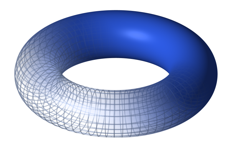
That is, the infinity symbol and a torus have the same connectivity between vertices; those vertices are just in different positions.
Mapping an object onto a 2D plane generally means finding a way to slice the object into pieces that fit onto that plane. However, a torus is, topologically speaking, equivalent to a plane. This plane is rolled into a tube, and bent around, so that each side connects to its opposing side directly. Therefore, mapping a texture onto this means reversing the process. The tube is cut at one end, creating a cylinder. Then, it is cut lengthwise, much like a car tire, and flattened out into a plane.
Exactly where those cuts need to be made is arbitrary. And because the specular texture mirrors perfectly in the S and T directions, it is not possible to tell exactly where the seams in the topology are. But they do need to be there.
What this does mean is that the vertices along the same have duplicate positions and normals. Because they have different texture coordinates, their shared positions and normals must be duplicated to match what OpenGL needs.
The best way to understand how the shininess texture affects the rendered result is to switch to the dark material with the 9 key. The plane also shows this a bit easier than the curved infinity symbol.
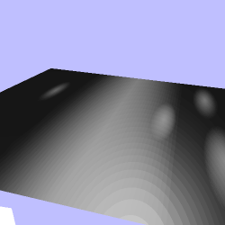
The areas with lower shininess, the bright areas, look like smudge marks. While the bright marks in the highly shiny areas only reflect light when the light source is very close to perfectly reflecting, the lower shininess areas will reflect light from much larger angles.
One interesting thing to note is how our look-up table works with the flat surface. Even at the highest resolution, 512 individual values, the lookup table is pretty poor; a lot of concentric rings are plainly visible. It looked more reasonable on the infinity symbol because it was heavily curved, and therefore the specular highlights were much smaller. On this flat surface, the visual artifacts become much more obvious. The Spacebar can be used to switch to a shader-based computation to see the correct version.
If our intent was to show a smudged piece of metal or highly reflective black surface, we could enhance the effect by also applying a texture that changed the specular reflectance. Smudged areas don't tend to reflect as strongly as the shiny ones. We could use the same texture mapping (ie: the same texture coordinates) and the specular texture would not even have to be the same size as our shininess texture.
There is one more thing to note about the shininess texture. The size of the texture is 1024x256 in size. The reason for that is that the texture is intended to be used on the infinity symbol. This object is longer in model space than it is around. By making the texture map 4x longer in the axis that is mapped to the S coordinate, we are able to more closely maintain the aspect ratio of the objects on the texture than the flat plane we see here. All of those oval smudge marks you see are in fact round in the texture. They are still somewhat ovoid and distorted on the infinity symbol though.
It is generally the job of the artist creating the texture mapping to ensure that the aspect ratio and stretching of the mapped object remains reasonable for the texture. In the best possible case, every texel in the texture maps to the same physical size on the object's surface. Fortunately for a graphics programmer, doing that isn't your job.
Unless of course your job is writing the tool that the artists use to help them in this process.