In all of the previous examples except for the translation one, we always combined the transformation with a translation operation. So the scale transform was not a pure scale transform; it was a scale and translate transformation matrix. The translation was there primarily so that we could see everything properly.
But these are not the only combinations of transformations that can be performed. Indeed, any combination of transformation operations is possible; whether they are meaningful and useful depends on what you are doing.
Successive transformations can be seen as doing successive multiplication operations. For example, if S is a pure scale matrix, T is a pure translation matrix, and R is a pure rotation matrix, then the shader can compute the result of a transformation as follows:
vec4 temp;
temp = T * position;
temp = R * temp;
temp = S * temp;
gl_Position = cameraToClipMatrix * temp;
In mathematical terms, this would be the following series of matrix operations: Final = C*S*R*T*position , where C is the camera-to-clip space transformation matrix.
This is functional, but not particularly flexible; the series of transforms is baked into the shader. It is also not particularly fast, what with having to do four vector/matrix multiplications for every vertex.
Matrix math gives us an optimization. Matrix math is not commutative: S*R is not the same as R*S . However, it is associative: (S*R)*T is the same as S*(R*T) . The usual grouping for vertex transformation is this: Final = C*(S*(R*(T*position))) . But this can easily be regrouped as: Final = (((C*S)*R)*T)*position .
This would in fact be slower for the shader to compute, since full matrix-to-matrix multiplication is much slower than matrix-to-vector multiplication. But the combined matrix (((C*S)*R)*T) is fixed for all of a given object's vertices. This can be computed on the CPU, and all we have to do is upload a single matrix to OpenGL. And since we're already uploading a matrix to OpenGL for each object we render, this changes nothing about the overall performance characteristics of the rendering (for the graphics hardware).
This is one of the main reasons matrices are used. You can build an incredibly complex transformation sequence with dozens of component transformations. And yet, all it takes for the GPU to use this to transform positions is a single vector/matrix multiplication.
As previously stated, matrix multiplication is not commutative. This means that the combined transform S*T is not the same as T*S . Let us explore this further. This is what these two composite transform matrices look like:
The transform S*T actually scales the translation part of the resulting matrix. This means that the vertices will not just get farther from each other, but farther from the origin of the destination space. It is the difference between these two transforms:

If you think about the order of operations, this makes sense. Even though one can think of the combined transform S*T as a single transform, it is ultimately a composite operation. The transformation T happens first; the object is translated into a new position.
What you must understand is that something special happens between S and T. Namely, that S is now being applied to positions that are not from model space (the space the original vertices were in), but are in post translation space. This is an intermediate coordinate system defined by T. Remember: a matrix, even a translation matrix, defines a full-fledged coordinate system.
So S now acts on the T-space position of the vertices. T-space has an origin, which in T-space is (0, 0, 0). However, this origin back in model space is the translation part of the matrix T. A scaling transformation matrix performs scaling based on the origin point in the space of the vertices being scaled. So the scaling matrix S will scale the points away from the origin point in T-space. Since what you (probably) actually wanted was to scale the points away from the origin point in model space, S needs to come first.
Orientation (rotation) matrices have the same issue. The orientation is always local to the origin in the current space of the positions. So a rotation matrix must happen before the translation matrix. Scales generally should happen before orientation; if they happen afterwards, then the scale will be relative to the new axis orientation, not the model-space one. This is fine if it is a uniform scale, but a non-uniform scale will be problematic.
There are reasons to put a translation matrix first. If the model-space origin is not the point that you wish to rotate or scale around, then you will need to perform a translation first, so that the vertices are in the space you want to rotate from, then apply a scale or rotation. Doing this multiple times can allow you to scale and rotate about two completely different points.
In more complex scenes, it is often desirable to specify the transform of one model relative to the model space transform of another model. This is useful if you want one object (object B) to pick up another object (object A). The object that gets picked up needs to follow the transform of the object that picked it up. So it is often easiest to specify the transform for object B relative to object A.
A conceptually single model that is composed of multiple transforms for multiple rendered objects is called a hierarchical model. In such a hierarchy, the final transform for any of the component pieces is a sequence of all of the transforms of its parent transform, plus its own model space transform. Models in this transform have a parent-child relationship to other objects.
For the purposes of this discussion, each complete transform for a model in the hierarchy will be called a node. Each node is defined by a specific series of transformations, which when combined yield the complete transformation matrix for that node. Usually, each node has a translation, rotation, and scale, though the specific transform can be entirely arbitrary. What matters is that the full transformation matrix is relative to the space of its parent, not camera space.
So if you have a node who's translation is (3, 0, 4), then it will be 3 X-units and 4 Z-units from the origin of its parent transform. The node itself does not know or care what the parent transform actually is; it simply stores a transform relative to that.
Technically, a node does not have to have a mesh. It is sometimes useful in a hierarchical model to have nodes that exist solely to position other, visible nodes. Or to act as key points for other purposes, such as identifying the position of the gun's muzzle to render a muzzle flash.
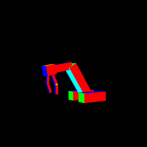
The Hierarchy tutorial renders a hierarchical model of an arm. This tutorial is interactive; the relative angles of the nodes can be changed with keyboard commands. The angles are bound within certain values, so the model will stop bending once these values are exceeded. These commands are as follows:
Table 6.1. Hierarchy Tutorial Key Commands
| Node Angle | Increase/Left | Decrease/Right |
|---|---|---|
| Base Spin | A | D |
| Arm Raise | W | S |
| Elbow Raise | R | F |
| Wrist Raise | T | G |
| Wrist Spin | Z | C |
| Finger Open/Close | Q | E |
The structure of the tutorial is very interesting and shows off a number of important data structures for doing this kind of rendering.
The class Hierarchy stores the information for our
hierarchy of nodes. It stores the relative positions for each node, as well as angle
information and size information for the size of each rectangle. The rendering code
in display simply does the usual setup work and calls
Hierarchy::Draw(), where the real work happens.
The Draw function looks like this:
Example 6.5. Hierarchy::Draw
void Draw()
{
    MatrixStack modelToCameraStack;

    glUseProgram(theProgram);
    glBindVertexArray(vao);

    modelToCameraStack.Translate(posBase);
    modelToCameraStack.RotateY(angBase);

    //Draw left base.
    {
        modelToCameraStack.Push();
        modelToCameraStack.Translate(posBaseLeft);
        modelToCameraStack.Scale(glm::vec3(1.0f, 1.0f, scaleBaseZ));
        glUniformMatrix4fv(modelToCameraMatrixUnif, 1, GL_FALSE,
            glm::value_ptr(modelToCameraStack.Top()));
        glDrawElements(GL_TRIANGLES, ARRAY_COUNT(indexData),
            GL_UNSIGNED_SHORT, 0);
        modelToCameraStack.Pop();
    }

    //Draw right base.
    {
        modelToCameraStack.Push();
        modelToCameraStack.Translate(posBaseRight);
        modelToCameraStack.Scale(glm::vec3(1.0f, 1.0f, scaleBaseZ));
        glUniformMatrix4fv(modelToCameraMatrixUnif, 1, GL_FALSE,
            glm::value_ptr(modelToCameraStack.Top()));
        glDrawElements(GL_TRIANGLES, ARRAY_COUNT(indexData),
            GL_UNSIGNED_SHORT, 0);
        modelToCameraStack.Pop();
    }

    //Draw main arm.
    DrawUpperArm(modelToCameraStack);

    glBindVertexArray(0);
    glUseProgram(0);
}
The program and VAO binding code should look familiar, but most of the code should be fairly foreign.
The MatrixStack object created in the very first line is a
class that is also a part of this project. It implements the concept of a
matrix stack. The matrix stack is a method for dealing
with transformations in hierarchical models.
A stack is a particular data structure concept. Stacks store a controlled sequence of objects. But unlike arrays, linked lists, or other general data structures, there are only 3 operations available to the user of a stack: push, pop, and peek. Push places a value on the top of the stack. Pop removes the value on the top of the stack, making the previous top the current top. And peek simply returns the current value at the top of the stack.
A matrix stack is, for the most part, a stack where the values are 4x4
transformation matrices. Matrix stacks do have a few differences from regular
stacks. C++ has an object, std::stack, that implements the
stack concept. MatrixStack is a wrapper around that object,
providing additional matrix stack functionality.
A matrix stack has a current matrix value. An initially constructed matrix stack
has an identity matrix. There are a number of functions on the matrix stack that
multiply the current matrix by a particular transformation matrix; the result
becomes the new current matrix. For example, the
MatrixStack::RotateX function multiplies the current
matrix by a rotation around the X axis by the given angle.
The MatrixStack::Push function takes the current matrix and
pushes it onto the stack. The MatrixStack::Pop function makes
the current matrix whatever the top of the stack is, and removes the top from the
stack. The effect of these is to allow you to save a matrix, modify the current
matrix, and then restore the old one after you have finished using the modified one.
And you can store an arbitrary number of matrices, all in a specific order. This is
invaluable when dealing with a hierarchical model, as it allows you to iterate over
each element in the model from root to the leaf nodes, preserving older transforms
and recovering them as needed.
In the Draw code, the translation is applied to the stack
first, followed by an X rotation based on the current angle. Note that the order of
operations is backwards from what we said previously. That's
because the matrix stack looks at transforms backwards. When we said earlier that
the rotation should be applied before the translation, that was with respect to the
position. That is, the equation should be
T*R*v
, where v is the position. What we meant was that R should be
applied to v before T. This means that R comes to the right of T.
Rather than applying matrices to vertices, we are applying matrices to each other. The matrix stack functions all perform right-multiplication; the new matrix being multiplied by the current is on the right side. The matrix stack starts with the identity matrix. To have it store T*R, you must first apply the T transform, which makes the current matrix the current matrix is I*T. Then you apply the R transform, making the current matrix I*T*R.
Right-multiplication is necessary, as the whole point of using the matrix stack is so that we can start at the root of a hierarchical model and save each node's transform to the stack as we go from parent to child. That simply would not be possible if matrix stacks left-multiplied, since we would have to apply the child transforms before the parent ones.
The next thing that happens is that the matrix is preserved by pushing it on the stack. After this, a translation and scale are applied to the matrix stack. The stack's current matrix is uploaded to the program, and a model is rendered. Then the matrix stack is popped, restoring the original transform. What is the purpose of this code?
What we see here is a difference between the transforms that need to be propagated to child nodes, and the transforms necessary to properly position the model(s) for rendering this particular node. It is often useful to have source mesh data where the model space of the mesh is not the same space that our node transform requires.
In our case, we do this because we know that all of our pieces are 3D rectangles. A 3D rectangle is really just a cube with scales and translations applied to them. The scale makes the cube into the proper size, and the translation positions the origin point for our model space.
Rather than have this extra transform, we could have created 9 or so actual rectangle meshes, one for each rendered rectangle. However, this would have required more buffer object room and more vertex attribute changes when these were simply unnecessary. The vertex shader runs no slower this way; it's still just multiplying by matrices. And the minor CPU computation time is exactly that: minor.
This concept is very useful, even though it is not commonly talked about to the point where it gets a special name. As we have seen, it allows easy model reuse, but it has other properties as well. For example, it can be good for data compression. There are ways to store values on the range [0, 1] or [-1, 1] in 16 or 8 bits, rather than 32-bit floating point values. If you can apply a simple scale+translation transform to go from this [-1, 1] space to the original space of the model, then you can cut your data in half (or less) with virtually no impact on visual quality.
Each section of the code where it uses an extra transform happens between a
MatrixStack::Push and
MatrixStack::Pop. This preserves the node's matrix, so that it
may be used for rendering with other nodes.
At the bottom of the base drawing function is a call to draw the upper arm. That function looks similar to this function: apply the model space matrix to the stack, push, apply a matrix, render, pop, call functions for child parts. All of the functions, to one degree or another, look like this. Indeed, they all looks similar enough that you could probably abstract this down into a very generalized form. And indeed, this is frequently done by scene graphs and the like. The major difference between the child functions and the root one is that this function has a push/pop wrapper around the entire thing. Though since the root creates a MatrixStack to begin with, this could be considered the equivalent.